Simulating and Visualizing Real-Life Events in Python with SimPy

Discrete Event Simulation (DES) has tended to be the domain of specialized products such as SIMUL8 and MATLAB/Simulink. However, while performing an analysis in Python for which I would have used MATLAB in the past, I had the itch to test whether Python has an answer for DES as well.

DES is a way to model real-life events using statistical functions, typically for queues and resource usage with applications in health care, manufacturing, logistics and others. The end goal is to arrive at key operational metrics such as resource usage and average wait times in order to evaluate and optimize various real-life configurations. SIMUL8 has a video depicting how emergency room wait times can be modelled, and MathWorks has a number of educational videos to provide an overview of the topic, in addition to a case study on automotive manufacturing. The SimPy library provides support for describing and running DES models in Python. Unlike a package such as SIMUL8, SimPy is not a complete graphical environment for building, executing and reporting upon simulations; however, it does provide the fundamental components to perform simulations and output data for visualization and analysis.

This article will first walk through a scenario and show how it can be implemented in SimPy. It will then look at three different approaches to visualizing the results: a Python-native solution (with Matplotlib and Tkinter), an HTML5 canvas-based approach, and an interactive AR/VR visualization. We will conclude by using our SimPy model to evaluate alternative configurations.

The Scenario

For our demonstration, I will use an example from some of my previous work: the entrance queue at an event. However, other examples that follow a similar pattern could be a queue at a grocery store or a restaurant that takes online orders, a movie theatre, a pharmacy, or a train station.

We will simulate an entrance that is served entirely by public transit: on a regular basis a bus will be dropping off several patrons who will then need to have their tickets scanned before entering the event. Some visitors will have badges or tickets they pre-purchased in advance, while others will need to approach seller booths first to purchase their tickets. Adding to the complexity, when visitors approach the seller booths, they will do so in groups (simulating a family/group ticket purchase); however, each person will need to have their tickets scanned separately. Figure 1 depicts the high-level layout of this scenario.

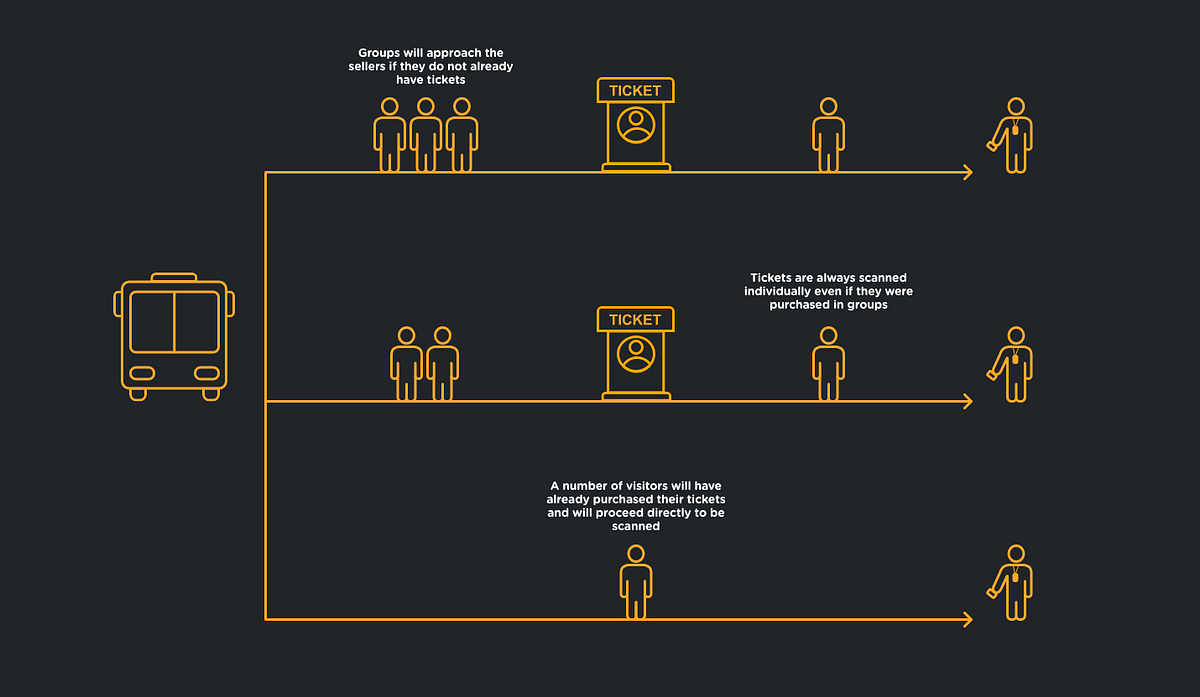
In order to simulate this, we will need to decide on how to represent these different events using probability distributions. The assumptions made in our implementation include:

• A bus will arrive on average 1 every 3 minutes. We will use an exponential distribution with a $\lambda$ of $1/3$ to represent this.
• Each bus will contain 100 +/- 30 visitors determined using a normal distribution ($\mu = 100$, $\sigma = 30$).
• Visitors will form groups of 2.25 +/- 0.5 people using a normal distribution ($\mu = 2.25$, $\sigma = 0.5$). We will round this to the closest whole number.
• We’ll assume that a fixed ratio of 40% of visitors will need to purchase tickets at the seller booths, another 40% will arrive with a ticket already purchased online, and 20% will arrive with staff credentials.
• Visitors will take one minute on average to exit the bus and walk to the seller booth (normal, $\mu = 1$, $\sigma = 0.25$), and another half minute to walk from the sellers to the scanners (normal, $\mu = 0.5$, $\sigma = 0.1$). For those skipping the sellers (tickets pre-purchased or staff with badges), we’ll assume an average walk of 1.5 minutes (normal, $\mu = 1.5$, $\sigma = 0.35$).
• Visitors will select the shortest line when they arrive, where each line has one seller or scanner.
• A sale requires 1 +/- 0.2 minutes to complete (normal, $\mu = 1$, $\sigma = 0.2$).
• A scan requires 0.05 +/- 0.01 minutes to complete (normal, $\mu = 0.05$, $\sigma = 0.01$).

With that in mind, let’s start with the output and work backwards from there.

Implementing the Simulation in SimPy

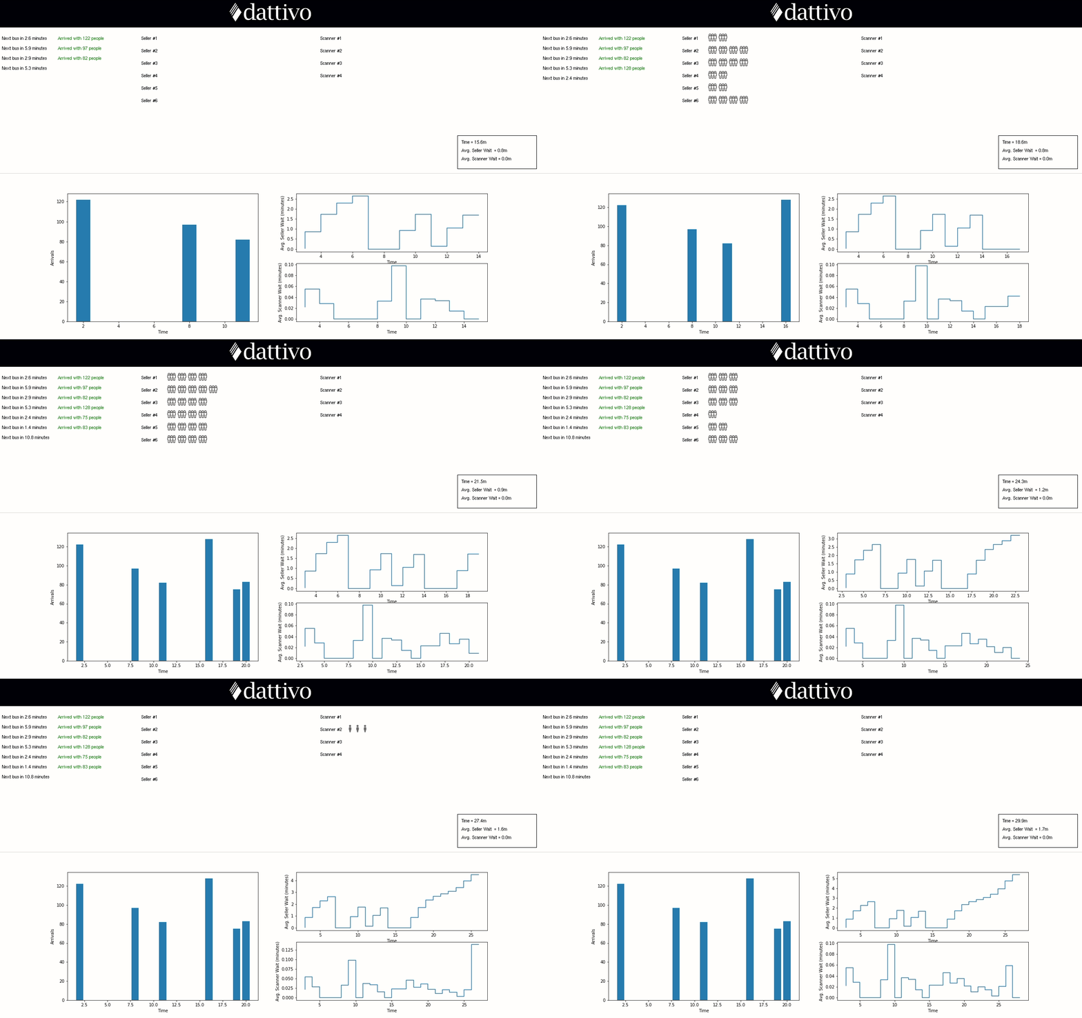
The graph on the left-hand side of Figure 2 represents the number of visitors arriving per minute and the graphs on the right-hand side represent the average time the visitors exiting the queue at that moment needed to wait before being served.

The repository with the complete runnable source can be found at github.com/dattivo/gate-simulation with the following snippets lifted from the simpy example.py file. In this section we will step through the SimPy-specific set up; however, note that the parts that connect to Tkinter for visualization are omitted to focus on the DES features of SimPy.

To begin, let’s start with the parameters of the simulation. The variables that will be most interesting to analyze are the number of seller lines (SELLER_LINES) and the number of sellers per line (SELLERS_PER_LINE) as well as their equivalents for the scanners (SCANNER_LINES and SCANNERS_PER_LINE). Also, note the distinction between the two possible queue/seller configurations: although the most prevalent configuration is to have multiple distinct queues that a visitor will select and stay at until they’re served, it has also become more mainstream in retail to see multiple sellers for one single line (e.g., quick checkout lines at general merchandise big box retailers).

BUS_ARRIVAL_MEAN = 3
BUS_OCCUPANCY_MEAN = 100
BUS_OCCUPANCY_STD = 30

PURCHASE_RATIO_MEAN = 0.4
PURCHASE_GROUP_SIZE_MEAN = 2.25
PURCHASE_GROUP_SIZE_STD = 0.50

TIME_TO_WALK_TO_SELLERS_MEAN = 1
TIME_TO_WALK_TO_SELLERS_STD = 0.25
TIME_TO_WALK_TO_SCANNERS_MEAN = 0.5
TIME_TO_WALK_TO_SCANNERS_STD = 0.1

SELLER_LINES = 6
SELLERS_PER_LINE = 1
SELLER_MEAN = 1
SELLER_STD = 0.2

SCANNER_LINES = 4
SCANNERS_PER_LINE = 1
SCANNER_MEAN = 1 / 20
SCANNER_STD = 0.01

With the configuration complete, let’s start the SimPy process by first creating an “environment”, all the queues (Resources), and running the simulation (in this case, until the 60-minute mark).

env = simpy.rt.RealtimeEnvironment(factor = 0.1, strict = False)

seller_lines = [ simpy.Resource(env, capacity = SELLERS_PER_LINE) for _ in range(SELLER_LINES) ]
scanner_lines = [ simpy.Resource(env, capacity = SCANNERS_PER_LINE) for _ in range(SCANNER_LINES) ]

env.process(bus_arrival(env, seller_lines, scanner_lines))

env.run(until = 60)

Note that we are creating a RealtimeEnvironment which is intended for running a simulation in near real-time, particularly for our intentions of visualizing this as it runs. With the environment set up, we generate our seller and scanner line resources (queues) that we will then in turn pass to our “master event” of the bus arriving. The env.process() command will begin the process as described in the bus_arrival() function depicted in Listing 3. This function is the top-level event from which all other events are dispatched. It simulates a bus arriving every BUS_ARRIVAL_MEAN minutes with BUS_OCCUPANCY_MEAN people on board and then triggers the selling and scanning processes accordingly.

def bus_arrival(env, seller_lines, scanner_lines):
    # Note that these unique IDs for busses and people are not required, but are included for eventual visualizations
    next_bus_id = 0
    next_person_id = 0
    while True:
        next_bus = random.expovariate(1 / BUS_ARRIVAL_MEAN)
        on_board = int(random.gauss(BUS_OCCUPANCY_MEAN, BUS_OCCUPANCY_STD))

        # Wait for the bus
        yield env.timeout(next_bus)

        people_ids = list(range(next_person_id, next_person_id + on_board))
        next_person_id += on_board
        next_bus_id += 1

        while len(people_ids) > 0:
            remaining = len(people_ids)
            group_size = min(round(random.gauss(PURCHASE_GROUP_SIZE_MEAN, PURCHASE_GROUP_SIZE_STD)), remaining)
            people_processed = people_ids[-group_size:]  # Grab the last `group_size` elements
            people_ids = people_ids[:-group_size]         # Reset people_ids to only those remaining

            # Randomly determine if this group is going to the sellers or straight to the scanners
            if random.random() > PURCHASE_RATIO_MEAN:
                env.process(scanning_customer(env, people_processed, scanner_lines, TIME_TO_WALK_TO_SELLERS_MEAN + TIME_TO_WALK_TO_SCANNERS_MEAN, TIME_TO_WALK_TO_SELLERS_STD + TIME_TO_WALK_TO_SCANNERS_STD))
            else:
                env.process(purchasing_customer(env, people_processed, seller_lines, scanner_lines))

Since this is the top-level event function, we see that all the work in this function is taking place within an endless while loop. Within the loop, we are “yielding” our wait time with env.timeout(). SimPy makes extensive use of generator functions which will return an iterator of the yielded values.

At the end of the loop, we are dispatching one of two events depending on whether we’re going directly to the scanners or if we’ve randomly decided that this group needs to purchase tickets first. Note that we are not yielding to these processes as that would instruct SimPy to complete each of these operations in sequence; instead, all those visitors exiting the bus will be proceeding to the queues concurrently.

Note that the people_ids list is being used so that each person is assigned a unique ID for visualization purposes. We are using the people_ids list as a queue of people remaining to be processed; as visitors are dispatched to their destinations, they are removed from the people_ids queue.

The purchasing_customer() function in Listing 4 simulates three key events: walking to the line, waiting in line, and then passing control to the scanning_customer() event (the same function that is called by bus_arrival() for those bypassing the sellers and going straight to the scanners). This function picks its line based on what is shortest at the time of selection.

def purchasing_customer(env, people_processed, seller_lines, scanner_lines):
    # Walk to the seller
    yield env.timeout(random.gauss(TIME_TO_WALK_TO_SELLERS_MEAN, TIME_TO_WALK_TO_SELLERS_STD))

    seller_line = pick_shortest(seller_lines)
    with seller_line[0].request() as req:
        yield req  # Wait in line

        yield env.timeout(random.gauss(SELLER_MEAN, SELLER_STD))  # Buy their tickets

        env.process(scanning_customer(env, people_processed, scanner_lines, TIME_TO_WALK_TO_SCANNERS_MEAN, TIME_TO_WALK_TO_SCANNERS_STD))

Finally, we need to implement the behaviour for the scanning_customer() in Listing 5. This is very similar to the purchasing_customer() function with one key difference: although visitors may arrive and walk together in groups, each person must have their ticket scanned individually. Consequently, you will see the scan timeout repeated for each scanned customer.

def scanning_customer(env, people_processed, scanner_lines, walk_duration, walk_std):
    # Walk to the scanner
    yield env.timeout(random.gauss(walk_duration, walk_std))

    # We assume that the visitor will always pick the shortest line
    scanner_line = pick_shortest(scanner_lines)
    with scanner_line[0].request() as req:
        yield req  # Wait in line

        # Scan each person's tickets
        for person in people_processed:
            yield env.timeout(random.gauss(SCANNER_MEAN, SCANNER_STD))

We pass the walk duration and standard deviation to the scanning_customer() function since those values will vary depending on whether the visitors walked directly to the scanners or if they stopped at the sellers first.

In order to visualize the data, we added a few global lists and dictionaries to track key metrics. For example, the arrivals dictionary tracks the number of arrivals by minute and the seller_waits and scan_waits dictionaries map the minute of the simulation to a list of wait times for those exiting the queues in those minutes. There is also an event_log list that we will use in the HTML5 Canvas animation in the next section. As key events take place (e.g., a visitor exiting a queue), the functions under the ANALYTICAL_GLOBALS heading in the simpy example.py file are called to keep these dictionaries and lists up to date.

Visualizing the Data using Tkinter (Native Python UI)

We used an ancillary SimPy event to send a tick event to the UI in order to update a clock, update the current wait averages and redraw the Matplotlib charts. The complete code can be found in the GitHub repository; however, Listing 6 provides a skeleton view of how these updates are dispatched from SimPy.

class ClockAndData:
    def __init__(self, canvas, x1, y1, x2, y2, time):
        # Draw the initial state of the clock and data on the canvas
        # ...
        self.canvas.update()

    def tick(self, time):
        # Re-draw the clock and data fields on the canvas. Also update the
        # Matplotlib charts (arrivals, seller waits, scanner waits).
        # ...

# ...

clock = ClockAndData(canvas, 1100, 320, 1290, 400, 0)

# ...

def create_clock(env):
    while True:
        yield env.timeout(0.1)
        clock.tick(env.now)

# ...

env.process(create_clock(env))

The visualization of the users moving to and from seller and scanner queues (the top portion of Figure 2) is represented using standard Tkinter logic. We created the QueueGraphics class to abstract the common parts of the seller and scanner queues. Methods from this class are coded into the SimPy event functions described in the previous section to update the canvas (e.g., sellers.add_to_line(1) where 1 is the seller number, and sellers.remove_from_line(1)). As future work, we could use an event handler at key points in the process so the SimPy simulation logic is not tightly coupled to the UI logic specific to this analysis.

Animating the Data Using HTML5 Canvas

As an alternate visualization, we wanted to export the events from the SimPy simulation and pull them into a simple HTML5 web application to visualize the scenario on a 2D canvas. We accomplished this by appending to an event_log list as SimPy events take place. In particular, the bus arrival, walk to seller, wait in seller line, buy tickets, walk to scanner, wait in scanner line, and scan tickets events are each logged as individual dictionaries that are then exported to JSON at the end of the simulation. You can see some sample outputs of this in the output directory.

We developed a quick proof-of-concept to show how these events can be translated into a 2D animation which you can experiment with here. You can see the source code for the animation logic in visualize.ts.

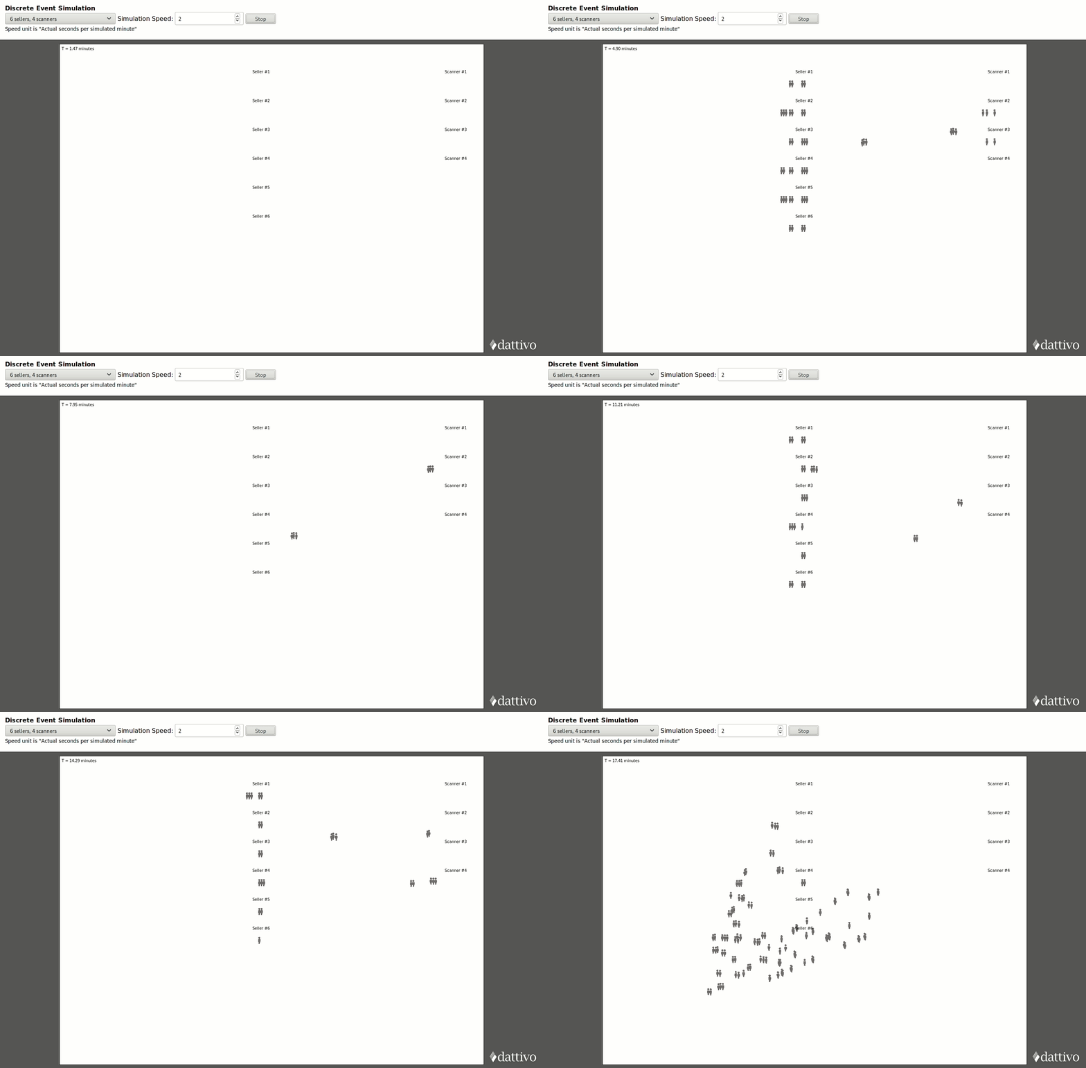
This visualization benefits from being animated; however, for practical purposes the Python-based Tkinter interface was quicker to assemble, and the Matplotlib graphs (which are arguably the most important part of this simulation) were also smoother and more familiar to set up in Python. That being said, there is value in seeing the behaviour animated, particularly when looking to communicate results to non-technical stakeholders.

Animating the Data Using Virtual Reality

Taking the canvas animation one step further, Matheus Ximenes and I worked together to put together the following AR/VR 3-D visualization using the same JSON simulation data that the HTML5 canvas is also using. We implemented this using React which we were already familiar with, and A-Frame which was surprisingly accessible and easy to learn.

Analyzing the Seller/Scanner Queue Configuration Alternatives

Although this example has been put together to demonstrate how a SimPy simulation can be created and visualized, we can still show a few examples to show how the average wait times depend on the configuration of the queues.

Let’s begin with the case demonstrated in the animations above: six sellers and four scanners with one seller and scanner per line (6/4). After 60 minutes, we see the average seller wait was 1.8 minutes and the average scanner wait was 0.1 minutes. From Figure 5, we see that the seller time peaks at almost a 6-minute wait.

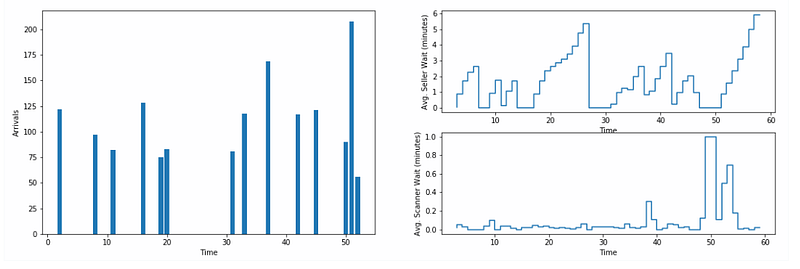
We can see that the sellers are consistently backed up; so, let’s see what happens if we add an extra four sellers, bumping the total up to 10.

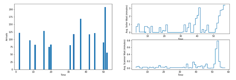
As expected, the average seller wait is reduced to 0.7 minutes and the maximum wait is reduced to be just over three minutes.

Now, let’s say that by reducing the price of online tickets, we’re able to boost the number of people arriving with a ticket by 35%. Initially, we assumed that 40% of all visitors need to buy a ticket, 40% have pre-purchased online, and 20% are staff and vendors entering with credentials. Therefore, with 35% more people arriving with tickets, we reduce the number of people needing to purchase down to 26%. Let’s simulate this with our initial 6/4 configuration.

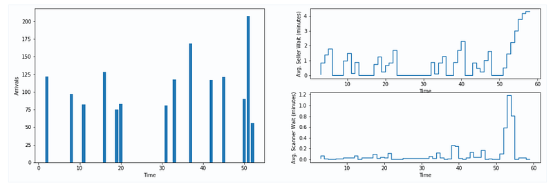
In this scenario, the average seller wait is reduced to 1.0 minutes with a maximum wait of just over 4 minutes. In this circumstance, increasing online sales by 35% had a similar effect to adding more seller queues to the average wait; if waiting time is the metric that we were most interested in reducing, then at that point we could consider which of these two options would have a stronger business case.

Conclusions and Future Work

The breadth of mathematical and analytical tools available for Python is formidable, and SimPy rounds out these capabilities to include discrete event simulations as well. Compared to commercially packaged tools such as SIMUL8, the Python approach does leave more to programming. Assembling the simulation logic and building a UI and measurement support from scratch may be clumsy for quick analyses; however, it does provide a lot of flexibility and should be relatively straightforward for anyone already familiar with Python. As demonstrated above, the DES logic provided by SimPy results in clean, easy-to-read code.

As mentioned, the Tkinter visualization is the most straightforward of the three demonstrated methods to work with, in particular with Matplotlib support included. The HTML5 canvas and AR/VR approaches have been handy for putting together a sharable and interactive visualization; however, their development was non-trivial.

One improvement that would be important to consider when comparing queue configurations is the seller/scanner utilization. Reducing the time in the queues is only one component of the analysis, as the percentage of the time that the sellers and scanners are sitting idle should also be considered in arriving at the most optimal solution. Additionally, it would also be interesting to add a probability that accounts for someone choosing not to enter if they see a queue that is too long.

Originally published at medium.com/data-science.