Fraud Classification in an Online Corporate Program
An online retailer I worked with had a special catalog that a selection of customers could access with a unique access code shared through their workplace to purchase items at reduced prices. There was some fraud that took place within this program with purchases made with stolen credit cards which were then charged back after-the-fact. Ideally, the client wanted to detect when one of these access codes had fallen into the wrong hands and invalidate it to prevent it from continuing to be used for fraud. This article shows how for this specific situation, introductory statistics is enough to create a robust fraud filter.
Background
There is one product – let’s call it Product X – that constitutes more than 80% of all fraud (by items purchased) but is not nearly as prevalent with non-fraudulent orders. In fact, we found that in the non-fraudulent order dataset, only 29.5% of all orders contain at least one Product X versus 99.25% of all known fraudulent orders. Since from a procedural perspective the client is able to review suspicious activity on a daily basis, this article investigates how we can help identify compromised access codes by looking at the percentage of their orders containing Product X over the past day.
Note that although the data has been inspired by a real-life data set, we have sanitized and simplified it for the purposes of this article.
The Dataset
Let’s begin by exporting all orders completed within the corporate program over a selected time period. We begin by grouping the data by the date purchased and the access code. We group by date since we’ll be looking for suspicious behaviour daily. Next, we filter this dataset to only include access codes on days where there are at least 15 orders. This filter has been applied since the ratio of orders containing at least one Product X can easily be skewed on a smaller sample size. Moreover, in looking at fraud patterns from the past, the tendency has been that the most popular (and widely shared) codes are most likely to be used for fraudulent purposes and they are likely to be used numerous times by the fraudster. Once grouped and filtered, we then extract the number of orders containing Product X and the total number of orders for each day/access code combination. The dataset will look something like Table 1 (the two grouped fields are the day and the access code):
| Day | Access Code | # Orders with Product X | # Orders | Ratio |
|---|---|---|---|---|
| 1 | ABCDEF | 12 | 48 | 0.25 |
| 1 | 123456 | 20 | 25 | 0.80 |
| 2 | ABCDEF | 8 | 42 | 0.19 |
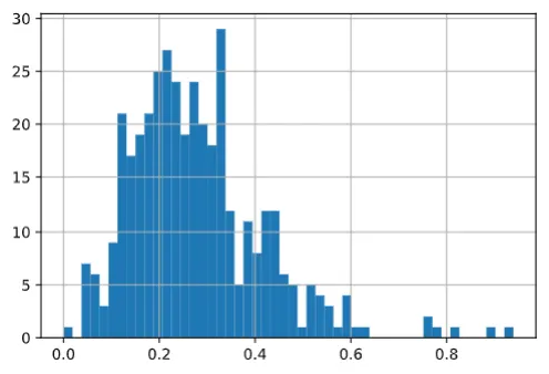
We’re interested in the ratio of orders with Product X since we know that an access code that skews higher is more likely to be fraud. We’ve represented the ratio in Figure 1 using a histogram.
In Theory
Given that this distribution has a lognormal shape, let’s test that by taking the log of the ratios and plotting it (Figure 2), then checking it against a quantile-quantile (QQ) graph (Figure 3).
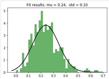
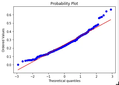
We can see that this looks “relatively normal”, especially closer to the mean. However, once we’re about two standard deviations in either direction, we see that we have fatter tails than a perfect normal curve.
If this were a perfectly normal distribution, then we could use the
normal percent-point function (also termed the quantile function) to
determine the value at which we can be 99% certain that there won’t be
more than a certain percentage of orders containing Product X. For
example, we know that for 99% certainty on a normal distribution, we
need to be 2.326 standard deviations above the mean (you can confirm
this by running scipy.stats.norm.ppf(0.99)). In our dataset above, we
have a mean of 0.2412 and a standard deviation of 0.109; consequently,
is 0.4947.
We can also see this visually using the cumulative distribution calculator at onlinestatbook.com. Again using a mean of 0.2412 and a standard deviation of 0.109, the probability of the value being greater than 0.4947 is represented by the shaded area in the right-hand side of the curve in Figure 4. The sum of the shaded area is 1% implying that there is only a 1% probability that the value will be greater than 0.4947.
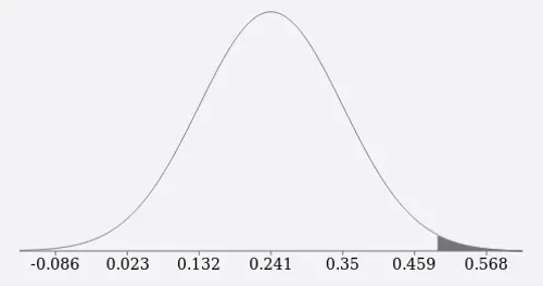
Therefore, reversing the log ratio of 0.4947 back to a regular percentage of 64% (), we can state with over 99% certainty that the ratio of orders containing Product X will not exceed 64% on any given day (for access codes having 15 or more orders on that day).
In Practice
We know that what was assumed in theory will not be the case in practice
due to the fat tails of the actual distribution. In actuality, six
day/access code combinations exceeded this threshold out of 387
day/access code combinations, or 1.55% versus the expected 1%. However,
of those six, five of them are the same access code that would later be
identified as being used for fraudulent orders (af8f8ac524 in
Table 2). Consequently,
it appears that this approach may even aid in identifying further fraud
that was not identified by a purely manual review. If that is the case,
then that will flatten out the fat tail as well.
With the non-fraudulent baseline established, let’s rerun the test on the entire dataset including known fraudulent orders. The number of day/access code combinations with a log value of 0.4947 or greater has increased from six to nine, with the three new values all being access codes that were used for fraudulent purposes.
| Day | Access Code | Num with Product X | Total | Log Prob of Having Product X |
|---|---|---|---|---|
| 6 | 060fb01292 | 21 | 27 | 0.575364 |
| 8 | 06c43e2450 | 36 | 45 | 0.587787 |
| 9 | 7831929800 | 29 | 42 | 0.525010 |
| 10 | 7831929800 | 27 | 31 | 0.626456 |
| 12 | af8f8ac524 | 40 | 53 | 0.562308 |
| 13 | af8f8ac524 | 35 | 43 | 0.595509 |
| 15 | af8f8ac524 | 56 | 69 | 0.594207 |
| 16 | af8f8ac524 | 91 | 94 | 0.677061 |
| 17 | af8f8ac524 | 31 | 33 | 0.662376 |
Results and Conclusions
Of all the codes in
Table 2, only
060fb01292 did not contain any known fraudulent orders. The codes
listed represent 89% of all known fraudulent orders in the corporate
program.
Although this scenario may not be generally applicable, the approach described in this article is demonstrably effective in this particular situation. By running a simple daily check for access codes having the ratio of its orders containing Product X greater than 64%, we’re able to identify 89% of all fraudulent orders within our dataset with very little noise (one false positive out of nine). These access codes can be suggested for staff to manually review on a daily basis; this will also greatly reduce the amount of time spent manually searching for suspicious transactions since this approach will focus the review on access codes that are most likely to contain fraud.
Moreover, consider that a purely manual review of the order list
resulted in the 7831929800 code being cancelled at the end of Day 10,
and the af8f8ac524 code being cancelled at the end of Day 17; with
this approach, the former could have been identified and cancelled one
day earlier, while the latter could have been cancelled five days
sooner.
One advantage of this approach is that it is difficult for fraudsters to adapt to. There are economic reasons why Product X is favoured by fraudsters, consequently it will be difficult for them to adapt to this strategy of fraud detection. For example, if we were looking at the quantity of Product X in a cart, or the total number of Product X purchased, then a fraudster could split their orders into smaller carts. However, since this approach looks at the ratio of orders having even just one Product X in their cart, it becomes more difficult for fraudsters to fly under the radar.
This approach underlines that knowing the intricacies of a dataset and the behaviours of the underlying actors can yield effective results with relatively straightforward statistical approaches. Although this ended up being a very simple approach, it does take a fair amount of domain knowledge and experimentation to arrive at an effective practical solution.